Contents
![[-]](/moniwiki/imgs/plugin/arrup.png "[-]")
![[+]](/moniwiki/imgs/plugin/arrdown.png "[+]")
- 1 회귀분석 기초
- 2 인과 관계 성립 조건
- 3 변수변환(Box-Cox변환)
- 4 단순회귀분석
- 5 중회귀분석
- 6 변수선택
- 7 더미변수
- 8 교호작용
- 9 다중공선성(multicollinearity)
- 10 회귀진단
- 11 두 회귀식의 비교
- 12 다변량 회귀분석
- 13 결과의 해석
- 14 표준화된 회귀계수(beta)
- 15 predict
- 16 마우스로 콕콕 찝어서 이상치 제거 후 회귀분석하기
- 17 coef의 신뢰구간
- 18 confidence, prediction level
- 19 R-squared
- 20 Adjusted R-squared
- 21 as.lm.nls
- 22 비모수 방법
- 23 오차 계산
- 24 t-sql로 구현한 단순회귀분석
- 25 Two-Stage Least Squares
- 26 참고자료
[edit]
1 회귀분석 기초 #
- '회귀(regression)' 개념은 19세기 말 영국의 생물통계학자 골튼(F.Galton)에 의해 처음 이용됨.
- 평균으로의 회귀.
- 변수 사이의 함수적 관계를 나타내는 수학적 회귀방정식을 구하고 독립변수를 특정한 값에 따른 종속변수의 값을 예측하는 기법
- 회귀분석은 서로 영향을 주고 받으면서 변화하는 인과관계를 갖는 두 변수 사이의 관계를 분석
- 산포도를 그려보면 회귀분석을 할 것인지 말 것인지 대략 결정할 수 있다. (양/음의 상관관계)
- 현상의 정량적 이해나 Y의 예측을 위하여 유효한 회귀 모델을 구축하는 것이 회귀분석의 주목적.
- 잔차(residual)분석: 모델검증
- 회귀진단: 특이한 이상치나 모수의 추정에 큰 영향을 주는 관측치 검출
- 목적변수가 양적변수일때 적용 가능
- 설명변수는 양적이거나 질적이거나 상관없으나, 질적변수는 데이터의 값이 0 또는 1만 취하는 더미변수를 도입하여 질적인 데이터를 변환해야 한다.
- 종속변수(y)는 정규분포라 가정
- 회귀식과 표준편차
- y = a + bx ± 1σ : 68.0%가 이 구간내에 들어온다.
- y = a + bx ± 2σ : 95.5%가 이 구간내에 들어온다.
- y = a + bx ± 3σ : 99.7%가 이 구간내에 들어온다.
- y = a + bx ± 1σ : 68.0%가 이 구간내에 들어온다.
[edit]
2 인과 관계 성립 조건 #
- 종속 변수와 독립 변수간에 상관 관계가 있어야 한다. (독립 변수가 변하면 종속 변수도 변해야 함)
- 독립 변수가 종속 변수보다 먼저 존재해야 한다. (시간의 우선성)
- 종속 변수와 독립 변수간의 상관 관계가 제3의 변수로 설명될 여지가 없어야 한다. (제3의 변수가 종속 변수를 설명해서는 안 된다)
[edit]
3 변수변환(Box-Cox변환) #
사용법은 다음과 같다.
library("TeachingDemos")
y <- rlnorm(500, 3, 2)
par(mfrow=c(2,2))
qqnorm(y)
qqnorm(bct(y,1/2))
qqnorm(bct(y,0))
hist(bct(y,0))

library("car")
y <- rlnorm(500, 3, 2)
hist(box.cox(y,0))
[edit]
4 단순회귀분석 #
근속년수와 연봉의 회귀분석
#x: 근속년수
x <- c(2,3,4,6,8,9,10,12,13,15,17,19,20,23,25,26,27,29,30,33)
#y: 연봉
y <- c(1500,1640,1950,2700,2580,3200,3750,2960,4200,3960,4310,3990,4010,4560,4800,5300,5050,5450,5950,5650)
result <- lm(y~x)
summary(result)
결과
Call:
lm(formula = y ~ x)

Residuals:
   Min     1Q Median     3Q    Max
-470.0 -290.8 -168.0  293.9  789.4

Coefficients:
            Estimate Std. Error t value Pr(>|t|)
(Intercept) 1708.117    173.489   9.846 1.13e-08 ***
x            130.960      9.089  14.409 2.52e-11 ***
---
Signif. codes:  0 ‘***’ 0.001 ‘**’ 0.01 ‘*’ 0.05 ‘.’ 0.1 ‘ ’ 1

Residual standard error: 386.6 on 18 degrees of freedom
Multiple R-squared: 0.9202,     Adjusted R-squared: 0.9158
F-statistic: 207.6 on 1 and 18 DF,  p-value: 2.522e-11
결과해석
- 회귀식: y = 130.960 * x + 1708.117
- 자유도: 18
- 결정계수(coefficient of determination): 0.9202(조정된 결정계수: 0.9158)는 이 모델이 92%를 설명함을 뜻함.
- Pr(>|t|) : F검정의 결과 (p-value) = 2.52e-11
- 귀무가설: 회귀식에 의미가 없다.
- 대립가설: 회귀식에 의미가 있다.
- p-value = 2.522e-11이므로 유의수준 0.05에서 대립가설 채택할 근거 있다. 즉, 회귀식에 의미가 있다.
- 귀무가설: 회귀식에 의미가 없다.
- 잔차분석
- 더빈 왓슨비(durbin-watson ration; 오차항간의 계열상관 유무조사)
- 바트렛의 검정(bartlett's test; 오차항의 분산의 균일성 조사)
- 잔차: Residual standard error: 386.6
- 더빈 왓슨비(durbin-watson ration; 오차항간의 계열상관 유무조사)
- 근속년수가 50년인 사람의 연봉은? 130.960 * 50 + 1708.117 = 8256.117 만원이다.
- 회귀식에 대입해서 잔차/표준편차 = 표준잔차, -2.5 <= 표준잔차 <= 2.5 면 정상치, 범위를 벗어나면 이상치일 가능성이 높다.
[edit]
5 중회귀분석 #
공던지기 결과과 악력, 신장, 체중의 중회귀분석
데이터
#x1:악력, x2:신장, x3:체중, y1:공던지기
x1 <- c(28,46,39,25,34,29,38,23,42,27,35,39,38,32,25)
x2 <- c(146,169,160,156,161,168,154,153,160,152,155,154,157,162,142)
x3 <- c(34,57,48,38,47,50,54,40,62,39,46,54,57,53,32)
y1 <- c(22,36,24,22,27,29,26,23,31,24,23,27,31,25,23)
data <- data.frame(y1,x1,x2,x3)
상관분석
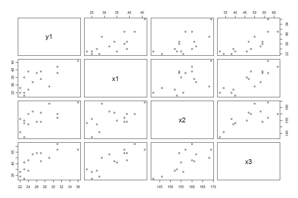
#시각적인 관찰(산포도)이 필요하면 pairs(data)하면 된다.
cov.wt(data, cor=T)

> cov.wt(data, cor=T)
$cov
         y1       x1       x2       x3
y1 16.31429 21.07143 20.01429 28.91429
x1 21.07143 48.66667 26.71429 53.64286
x2 20.01429 26.71429 52.25714 45.60000
x3 28.91429 53.64286 45.60000 82.54286

$center
       y1        x1        x2        x3
 26.20000  33.33333 156.60000  47.40000

$n.obs
[1] 15

$cor
          y1        x1        x2        x3
y1 1.0000000 0.7478150 0.6854618 0.7879319
x1 0.7478150 1.0000000 0.5297304 0.8463624
x2 0.6854618 0.5297304 1.0000000 0.6943082
x3 0.7879319 0.8463624 0.6943082 1.0000000

>
결과해석- x1(악력)과 x3(체중)의 상관계수가 가장 높다. 0.8463624
- x1(악력)과 x2(신장)의 상관계수가 가장 낮다. 0.5297304
- 공던지기(y1)와 상관계수가 높은 순서는 체중(x3), 악력(x1), 신장(x2)의 순이다.
회귀분석
summary(lm(y1~x1+x2+x3))
> summary(lm(y1~x1+x2+x3))

Call:
lm(formula = y1 ~ x1 + x2 + x3)

Residuals:
    Min      1Q  Median      3Q     Max
-3.9976 -1.3822  0.3611  1.1549  3.9291

Coefficients:
            Estimate Std. Error t value Pr(>|t|)
(Intercept) -13.2173    17.6038  -0.751    0.469
x1            0.2014     0.1842   1.093    0.298
x2            0.1710     0.1316   1.300    0.220
x3            0.1249     0.1667   0.750    0.469

Residual standard error: 2.532 on 11 degrees of freedom
Multiple R-squared: 0.6913,     Adjusted R-squared: 0.6072
F-statistic: 8.213 on 3 and 11 DF,  p-value: 0.003774

>
결과해석- 결정계수: 0.6913 (조정: 0.6072), 회귀식은 약 69%를 설명함.
- p-value: 0.003774으로 유의수준 0.05에서 대립가설을 채택. 즉, 회귀식은 유의함.
- 회귀식: y1 = -13.2173 + x1 * 0.2014 + x2 * 0.1710 + x3 * 0.1249
- Pr(>|t|)가 모두 0.05를 넘는 수준이다. 별로 안 좋다.
- 목적변수에 대한 각 설명변수의 영향력(t)
- 악력(x1) = 1.093
- 신장(x2) = 1.300
- 체중(x3) = 0.750
- 신장이 공던지기(y1)에 가장 많은 영향력을 끼치고 있다.
- 악력(x1) = 1.093
- 편회귀계수의 유의성 판정(F)
- 악력(x1) = 0.298
- 신장(x2) = 0.220
- 체중(x3) = 0.469
- 모두 0.05를 넘는다. 다중공선성을 의심해야 한다. 교호작용이 있는지도 봐야 한다.
- 악력(x1) = 0.298
[edit]
6 변수선택 #
- 변수를 잘못 선택하면?
- 추정의 정밀도가 나빠진다.
- y의 예측치는 편의를 갖게되고, 오차분산의 추정치는 과대평가하게 된다.
- 다중공선성(multicollinearity)의 문제 발생
- 추정의 정밀도가 나빠진다.
- 변수선택방법
- 전진선택(forward selection)
- 후진소거(backward elimination)
- 둘다(전진선택, 후진소거)
- 전진선택(forward selection)
- 이는 로지스틱 회귀분석의
![[http]](/moniwiki/imgs/http.png) 여기에 사용법이 기술되어 있다.
여기에 사용법이 기술되어 있다.
library("MASS")
fit <- lm(y1~x1+x2+x3,data=mydata)
step <- stepAIC(fit, direction="both")
step$anova # display results
[edit]
7 더미변수 #
- 만약 성별, 요일과 같은 변수가 회귀식에 포함되어야 하면 더미변수를 추가해야 함.
- p종류의 범주가 있으면 p-1개의 더미변수가 필요함.
- 성별은 2가지라 0, 1로 그냥 세팅하면 되지만 요일은 다음과 같이 해야 함.
- y = x + x1 + x2 + x3 + x4 + x5 + x6
	x1	x2	x3	x4	x5	x6
월	0	0	0	0	0	0
화	1	0	0	0	0	0
수	0	1	0	0	0	0
목	0	0	1	0	0	0
금	0	0	0	1	0	0
토	0	0	0	0	1	0
일	0	0	0	0	0	1
[edit]
8 교호작용 #
가끔씩 두 개 이상의 변수 짬뽕으로 결과에 영향을 끼치는 경우가 있다.
교호작용이 없는 모델
m1 <- lm(formula=Height~Girth + Volume, data=trees)
summary(m1)
> summary(m1)

Call:
lm(formula = Height ~ Girth + Volume, data = trees)

Residuals:
    Min      1Q  Median      3Q     Max
-9.7855 -3.3649  0.5683  2.3747 11.6910

Coefficients:
            Estimate Std. Error t value Pr(>|t|)
(Intercept)  83.2958     9.0866   9.167 6.33e-10 ***
Girth        -1.8615     1.1567  -1.609   0.1188
Volume        0.5756     0.2208   2.607   0.0145 *
---
Signif. codes:  0 ‘***’ 0.001 ‘**’ 0.01 ‘*’ 0.05 ‘.’ 0.1 ‘ ’ 1

Residual standard error: 5.056 on 28 degrees of freedom
Multiple R-squared:  0.4123,	Adjusted R-squared:  0.3703
F-statistic:  9.82 on 2 and 28 DF,  p-value: 0.0005868
교호작용이 있는 모델
m2 <- lm(formula=Height~Girth + Volume + Girth:Volume, data=trees)
summary(m2)
> summary(m2)

Call:
lm(formula = Height ~ Girth + Volume + Girth:Volume, data = trees)

Residuals:
    Min      1Q  Median      3Q     Max
-6.7781 -3.5574 -0.1512  2.3631 10.5879

Coefficients:
             Estimate Std. Error t value Pr(>|t|)
(Intercept)  75.40148    8.49147   8.880  1.7e-09 ***
Girth        -2.29632    1.03601  -2.217 0.035270 *
Volume        1.86095    0.47932   3.882 0.000604 ***
Girth:Volume -0.05608    0.01909  -2.938 0.006689 **
---
Signif. codes:  0 ‘***’ 0.001 ‘**’ 0.01 ‘*’ 0.05 ‘.’ 0.1 ‘ ’ 1

Residual standard error: 4.482 on 27 degrees of freedom
Multiple R-squared:  0.5546,	Adjusted R-squared:  0.5051
F-statistic: 11.21 on 3 and 27 DF,  p-value: 5.898e-05
두 변수의 교호작용은 곱하기(Girth*trees)다. 아래의 A, B의 결과는 같다.
A
fitted(m2)
B
coef(m2)[1] + coef(m2)[2]*trees$Girth + coef(m2)[3]*trees$Volume + coef(m2)[4]*trees$Girth*trees$Volume
[edit]
9 다중공선성(multicollinearity) #
- 설명변수 사이에 선형관계가 두 개 이상 있을 때 다중공선성이 있다고 말한다.
- 상관분석(R함수: cov.wt())해서 상관계수가 1에 가까운 설명변수를 버린다.
- 다중공선성 진단
- 설명변수 x1, x2, x3, x4가 있을 경우
- x1 ~ x2 + x3 + x4 -> 상관계수 R1 -> 허용도(tolerance) = 1 - R1^2
- x2 ~ x1 + x3 + x4 -> 상관계수 R2 -> 허용도(tolerance) = 1 - R2^2
- x3 ~ x1 + x2 + x4 -> 상관계수 R3 -> 허용도(tolerance) = 1 - R3^2
- x4 ~ x1 + x2 + x3 -> 상관계수 R4 -> 허용도(tolerance) = 1 - R4^2
- (1 - Rj^2) = 허용도가 작을 때는 Rj가 1에 가까우므로 xj는 다른 설명변수의 선형결합으로 표현할 수 있다.
- 분산팽창계수(VIF: variance inflation factor) = 1 / (1 - Ri^2)가 10보다 크면 다중공선성이 존재한다고 경험적으로 판단함.
- VIP = 1 / (1 - Rj^2) = 1 / (1 - 0.7432^2) = 2.233869
- 설명변수 x1, x2, x3, x4가 있을 경우
#install.packages("Design",dependencies=T)
library("Design")
result <- lm(y1~x1+x2+x3)
vif(result)

> library("Design")
요구된 패키지 Hmisc를 로드중입니다

다음의 패키지를 첨가합니다: 'Hmisc'


        The following object(s) are masked from package:base :

         format.pval,
         round.POSIXt,
         trunc.POSIXt,
         units

요구된 패키지 survival를 로드중입니다
요구된 패키지 splines를 로드중입니다

다음의 패키지를 첨가합니다: 'survival'


        The following object(s) are masked from package:Hmisc :

         untangle.specials

Design library by Frank E Harrell Jr

Type library(help='Design'), ?Overview, or ?Design.Overview')
to see overall documentation.


다음의 패키지를 첨가합니다: 'Design'


        The following object(s) are masked from package:survival :

         Surv,
         survfit

> result <- lm(y1~x1+x2+x3)
> vif(result)
      x1       x2       x3
3.607546 1.975832 5.010688
>
결과해석- x1의 VIF: 3.607546
- x2의 VIF: 1.975832
- x3의 VIF: 5.010688
- VIF가 10이 넘지 않으므로 다중공선성은 없는 것으로 판단된다.
[edit]
10 회귀진단 #
잔차는..
- 정규분포를 따라야하고,
- 분산이 일정하고,
- 특별한 추세를 보이지 않아야 한다.
par(mfrow=c(2,2))
plot(lm(formula = y1 ~ x1 + x2 + x3 + x1:x2))
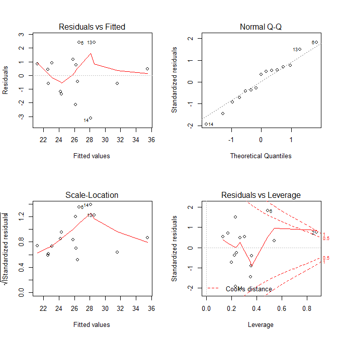
- 좌상: 예측값, 잔차 --> 0으로부터 고르게 분포하고 있는가?
- 우상: 표준화된 잔차의 Q-Q Plot --> 정규성을 띄는가?
- 좌하: 예측값, 스튜던트 잔차(표준화된 잔차)의 제곱근 --> 직선에 가까워야 한다.. 분산이 일정하지 않음을 의심해야 함.
- 우하: 레버러지와 스튜던트 잔차 plot --> rs = (k + 1 / n) * 2; k = predictor의 숫자, n = sample_size; rs보다 크가면 outlier
> out <- lm(formula = y1 ~ x1 + x2 + x3 + x1:x2)
> shapiro.test(resid(out))

        Shapiro-Wilk normality test

data:  resid(out)
W = 0.9669, p-value = 0.8099

>
결과에서 볼 수 있듯이 p-value = 0.8099로 '정규분포와 차이가 없다'라는 귀무가설을 조낸 지지한다. 즉, 잔차는 정규분포를 따른다.등분산성
브로슈-파간 테스트(Breusch- Pagan Test)로 등분산인지 알아본다.
브로슈-파간 테스트(Breusch- Pagan Test)로 등분산인지 알아본다.
> library("lmtest")
> bptest(out)

        studentized Breusch-Pagan test

data:  out
BP = 5.6201, df = 4, p-value = 0.2294

>
p-value가 0.2294로 유의수준 0.05에서 귀무가설 지지한다. 즉, 등분산이다. 만약 이분산(heterogenous variance)일 경우 가중최소제곱(weighted least squares; nls()사용)의 사용. 변수변환을 통해 교정할 수도 있다. > out <- lm(formula = y1 ~ x1 + x2 + x3 + x1:x2, weights=I(x1^(2)))
> summary(out)
Call:
lm(formula = y1 ~ x1 + x2 + x3 + x1:x2, weights = I(x1^(2)))
Residuals:
Min 1Q Median 3Q Max
-106.194 -34.272 4.358 30.456 85.645
Coefficients:
Estimate Std. Error t value Pr(>|t|)
(Intercept) 206.98239 62.41049 3.316 0.00779 **
x1 -6.74461 1.84209 -3.661 0.00438 **
x2 -1.25865 0.40492 -3.108 0.01109 *
x3 0.44112 0.13692 3.222 0.00915 **
x1:x2 0.04199 0.01105 3.800 0.00349 **
---
Signif. codes: 0 ‘***’ 0.001 ‘**’ 0.01 ‘*’ 0.05 ‘.’ 0.1 ‘ ’ 1
Residual standard error: 61.32 on 10 degrees of freedom
Multiple R-squared: 0.8834, Adjusted R-squared: 0.8368
F-statistic: 18.94 on 4 and 10 DF, p-value: 0.0001167
독립성
> library("lmtest")
> dwtest(out)

        Durbin-Watson test

data:  out
DW = 2.3524, p-value = 0.7083
alternative hypothesis: true autocorrelation is greater than 0

>
- d통계량
- 0 : 양의 자기상관, p-value = 1
- 2 : 독립, p-value = 0
- 4 : 음의 자기상관, p-value = -1
- 0 : 양의 자기상관, p-value = 1
- 대략적으로 DW값이 1보다 작거나 3보다 크면 자기상관이 확실히 있다고 판달할 수 있으며, 1.5~2.5 사이에 있을 경우 독립이라고 판단
- 대략 독립.
![[https]](/moniwiki/imgs/https.png)
[edit]
11 두 회귀식의 비교 #
data(airquality)
lm1<-lm(Ozone~.,airquality) # full model
lm2<-lm(Ozone~Solar.R+Wind +Month+Day,airquality) # reduced model
anova(lm2,lm1)
[edit]
12 다변량 회귀분석 #
여기에서는 그냥 lm()함수의 다변량 회귀분석의 사용방법만 보자.
y2 <- x1 #x1을 종속변수라 가정하고...
summary(lm(cbind(y1,y2)~x2+x3))

> y2 <- x1
> summary(lm(cbind(y1,y2)~x2+x3))
Response y1 :

Call:
lm(formula = y1 ~ x2 + x3)

Residuals:
    Min      1Q  Median      3Q     Max
-3.5060 -1.5862  0.2502  0.8539  5.3777

Coefficients:
            Estimate Std. Error t value Pr(>|t|)
(Intercept)  -9.8745    17.4765  -0.565   0.5825
x2            0.1493     0.1311   1.139   0.2770
x3            0.2678     0.1043   2.567   0.0247 *
---
Signif. codes:  0 ‘***’ 0.001 ‘**’ 0.01 ‘*’ 0.05 ‘.’ 0.1 ‘ ’ 1

Residual standard error: 2.552 on 12 degrees of freedom
Multiple R-squared: 0.6578,     Adjusted R-squared: 0.6008
F-statistic: 11.53 on 2 and 12 DF,  p-value: 0.001605


Response y2 :

Call:
lm(formula = y2 ~ x2 + x3)

Residuals:
    Min      1Q  Median      3Q     Max
-5.4716 -1.9151 -0.2964  1.9562  7.1935

Coefficients:
            Estimate Std. Error t value Pr(>|t|)
(Intercept)  16.5997    27.1675   0.611 0.552589
x2           -0.1079     0.2038  -0.529 0.606186
x3            0.7095     0.1622   4.375 0.000904 ***
---
Signif. codes:  0 ‘***’ 0.001 ‘**’ 0.01 ‘*’ 0.05 ‘.’ 0.1 ‘ ’ 1

Residual standard error: 3.967 on 12 degrees of freedom
Multiple R-squared: 0.7228,     Adjusted R-squared: 0.6766
F-statistic: 15.65 on 2 and 12 DF,  p-value: 0.0004537


>
[edit]
13 결과의 해석 #
뭘 또 이렇게까지나 해야 하는지?? 안 해도 되는거 같으다.
> summary(model)

Call:
lm(formula = 통계 ~ 수학 + 결석, data = result)

Residuals:
   Min     1Q Median     3Q    Max
-5.348 -2.274 -1.276  2.954  5.673

Coefficients:
            Estimate Std. Error t value Pr(>|t|)
(Intercept)  53.6832    14.1808   3.786  0.00431 **
수학          0.6073     0.1984   3.062  0.01353 *
결석         -1.9346     0.9144  -2.116  0.06348 .
---
Signif. codes:  0 ‘***’ 0.001 ‘**’ 0.01 ‘*’ 0.05 ‘.’ 0.1 ‘ ’ 1

Residual standard error: 3.721 on 9 degrees of freedom
Multiple R-squared: 0.8289,     Adjusted R-squared: 0.7909
F-statistic:  21.8 on 2 and 9 DF,  p-value: 0.0003544
- 회귀직선이 y=통계, x1=수학, x2=결석 이라면, y = 53.6832 + 0.6073x1 + -1.9346x2 으로 추정된다.
- -1.9346x2으로 마이너스(-)값을 가진다는 것은 결석을 할 수록 통계성적이 나빠진다는 것을 의미한다.
- 'β1=0'이라는 귀무가설에 대한 T 검정통계량은 3.062이며, 이것은 P값은 0.01353으로 유의수준 0.05에서는 귀무가설을 기각하게 된다. 즉, 유의미한 값이다.
- 결정계수 R2은 아래의 anova(분산분석)의 결과에서 R2 = (541.69 + 61.97)/(541.69 + 61.97 + 124.59) = 0.8289186405이고, 조정된 R2값은 0.7909 이다. 즉, 통계성적은 수학성적과 결석횟수 2개의 변수에 의해 약 83%가 설명되어진다.
- F 검정통계량은 21.8이며, F분포표의 α = 0.05, v1=2, v2=9의 값은 4.26이다. 즉, 21.8 > 4.26 이므로 귀무가설(β1=β2=0)은 기각한다. 즉, 유의미한 값이다. p-value가 나오므로 F분포표를 볼 필요는 없다. 유의수준 0.05 > 0.0003544 이므로 귀무가설을 기각하면 된다.
- p-value가 작으면 대립가설을 지지하고, 커지면 귀무가설을 지지한다. 0.0003544는 귀무가설이 맞다고 가정했을 경우 얻어진 검정통계량보다 더 극단적인 결과가 나올 확률이다. 즉, 통계적인 수치에 근거하여 의사결정을 했을 때에 오류(1종 오류)가 나올 확률.
- 유의수준 0.05라는 것은 95%만 평균에 가까운 정상으로 생각하고, 평균가 멀리 떨어진 5%는 비정상으로 생각한다는 것이다.
> anova(model) #자유도, 제곱합, 제곱평균 F값,
Analysis of Variance Table

Response: 통계
          Df Sum Sq Mean Sq F value    Pr(>F)
수학       1 541.69  541.69 39.1297 0.0001487 ***
결석       1  61.97   61.97  4.4762 0.0634803 .
Residuals  9 124.59   13.84
---
Signif. codes:  0 ‘***’ 0.001 ‘**’ 0.01 ‘*’ 0.05 ‘.’ 0.1 ‘ ’ 1
| 요인 | 제곱합 | 자유도 | 제곱평균 | F비 |
| 회귀 | 603.66 | 11 | 301.83 | 21.802950 |
| 잔차 | 124.59 | 9 | 13.84 | |
| 계 | 728.25 | 11 |
- F 검정통계량은 21.8이며, F분포표의 α = 0.05, v1=2, v2=9의 값은 4.26이다. 즉, 21.8 > 4.26 이므로 귀무가설(β1=β2=0)은 기각한다. 즉, 유의미한 값이다.
- 결정계수 R2은 아래의 R2 = 603.66/728.25 = 0.82891864 이다.
- 자유도란 자유로운 정도. 랜덤한 정도. 수식에 의해 자유가 제한되지 않는 정도인데 보통 표본의 개수를 의미한다.
fit <- lm(Volume ~ Girth + Height, data=trees)
f <- summary(fit)$fstatistic
pf(f[1],f[2],f[3],lower.tail=F)
참고: 95% 신뢰구간
confint(model, level=0.95)

                2.5 %     97.5 %
(Intercept)  502.5676  524.66261
poly(q, 3)1 1919.2739 2232.52494
poly(q, 3)2 -264.6292   48.62188
poly(q, 3)3  707.3999 1020.65097
[edit]
14 표준화된 회귀계수(beta) #
- B : 비표준화 회귀계수
- beta : 표준화 회귀계수
model <- lm(Girth ~ Height + Volume, data=trees)
summary(model)
결과
> summary(model)

Call:
lm(formula = Girth ~ Height + Volume, data = trees)

Residuals:
     Min       1Q   Median       3Q      Max
-1.34288 -0.56696 -0.08628  0.80283  1.11642

Coefficients:
            Estimate Std. Error t value Pr(>|t|)
(Intercept) 10.81637    1.97320   5.482 7.45e-06 ***
Height      -0.04548    0.02826  -1.609    0.119
Volume       0.19518    0.01096  17.816  < 2e-16 ***
---
Signif. codes:  0 ‘***’ 0.001 ‘**’ 0.01 ‘*’ 0.05 ‘.’ 0.1 ‘ ’ 1

Residual standard error: 0.7904 on 28 degrees of freedom
Multiple R-squared:  0.9408,	Adjusted R-squared:  0.9366
F-statistic: 222.5 on 2 and 28 DF,  p-value: < 2.2e-16
각각의 계수(B)는 나오는데, 어떤 변수가 더 큰 영향을 끼치는지 알 수 없다.
이런 경우 beta를 보면되는데, lm결과에 나오지 않는다. 다음과 같이 하면 된다.
이런 경우 beta를 보면되는데, lm결과에 나오지 않는다. 다음과 같이 하면 된다.
#install.packages("QuantPsyc")
library("QuantPsyc")
lm.beta(model)
결과
> lm.beta(model)
     Height      Volume
-0.09235166  1.02236871
Volume이 거의 모든 영향을 끼쳤다. 물론 beta를 보기 전에 Height 변수는 모델에서 제거 되었을 것이다.[edit]
15 predict #
y <- seq(1: nrow(x1))
dau <- x1$dau
fit <- lm(dau ~ poly(y, 3))
summary(fit)

plot(dau~y)
lines(y, predict(fit, data.frame(y=y)), col="purple")

newdata <- data.frame(y = seq(139,145))
predict(fit, newdata)

out <- lm(dau~y + I(y^2) + I(y^3))
summary(out)

p <- 145
3.131e+06 - p*2.637e+04 + (p^2) * 2.438e+02 - (p^3)*1.138e+00
[edit]
16 마우스로 콕콕 찝어서 이상치 제거 후 회귀분석하기 #
plot(y ~ x, data=df)
notin <- identify(df$x, df$y, labels=row.names(df))

fit <- lm(y ~ x - 1, data=df[!rownames(df) %in% notin,])
summary(fit)

plot(y ~ x, data=df[!rownames(df) %in% notin,])
abline(fit)
[edit]
17 coef의 신뢰구간 #
se <- sqrt(diag(vcov(bu.model)))[2]
ci.upr <-  coef(bu.model)[2] + 1.96*se
ci.lwr <-  coef(bu.model)[2]  - 1.96*se
[edit]
18 confidence, prediction level #
- interval = "confidence"는 평균적인 것, 즉, 오차항(intercept)을 고려치 않아(0으로 가정) 범위가 prediction에 비해 좁다.
- interval = "prediction"은 single value에 대한 것, 즉, 오차항(intercept)가 고려해야 함
# Make up some data
x <- seq(0, 1, length.out = 20)
y <- x^2 + rnorm(20)

# fit a quadratic
model <- lm(y ~ I(x^2))
fitted <- predict(model, interval = "confidence", level=.95)

# plot the data and the fitted line
plot(x, y)
lines(x, fitted[, "fit"])

# now the confidence bands
lines(x, fitted[, "lwr"], lty = "dotted")
lines(x, fitted[, "upr"], lty = "dotted")
[edit]
19 R-squared #
R^2의 의미
- 회귀식이 설명하는 변동량
- 실제값과 예측값의 상관관계(R^2는 피어슨 상관계수의 제곱)
d <- data.frame(y=(1:10)^2,x=1:10)
model <- lm(y~x,data=d)
d$prediction <- predict(model,newdata=d)

#R-squared
1-sum((d$prediction-d$y)^2)/sum((mean(d$y)- d$y)^2)
독립변수가 많아지면 R^2가 커지는 경향이 있다. 그래서 조정된 R^2를 사용한다.
여러 독립변수를 사용한 회귀식간의 비교는 조정된 R^2로 비교해야 한다.
조정된 R^2은 다음과 같이 구한다.
여러 독립변수를 사용한 회귀식간의 비교는 조정된 R^2로 비교해야 한다.
조정된 R^2은 다음과 같이 구한다.
m <- lm(Girth~Height, trees)
summary(m)
> summary(m)

Call:
lm(formula = Girth ~ Height, data = trees)

Residuals:
    Min      1Q  Median      3Q     Max
-4.2386 -1.9205 -0.0714  2.7450  4.5384

Coefficients:
            Estimate Std. Error t value Pr(>|t|)
(Intercept) -6.18839    5.96020  -1.038  0.30772
Height       0.25575    0.07816   3.272  0.00276 **
---
Signif. codes:  0 ‘***’ 0.001 ‘**’ 0.01 ‘*’ 0.05 ‘.’ 0.1 ‘ ’ 1

Residual standard error: 2.728 on 29 degrees of freedom
Multiple R-squared:  0.2697,	Adjusted R-squared:  0.2445
F-statistic: 10.71 on 1 and 29 DF,  p-value: 0.002758
[edit]
20 Adjusted R-squared #
n <- length(trees$Girth) #표본수
p <- 1                   #독립변수수
R2 <- cor(trees$Girth, fitted(m))^2 #R-squared
1 - ((n-1)*(1-R2)/(n-p-1)) #Adjusted R-squared
[edit]
21 as.lm.nls #
as.lm.nls <- function(object, ...) {
    if (!inherits(object, "nls")) {
        w <- paste("expected object of class nls but got object of class:",
			paste(class(object), collapse = " "))
		warning(w)
	}

	gradient <- object$m$gradient()
	if (is.null(colnames(gradient))) {
		colnames(gradient) <- names(object$m$getPars())
	}

	response.name <- if (length(formula(object)) == 2) "0" else
		as.character(formula(object)[[2]])

	lhs <- object$m$lhs()
	L <- data.frame(lhs, gradient)
	names(L)[1] <- response.name

	fo <- sprintf("%s ~ %s - 1", response.name,
		paste(colnames(gradient), collapse = "+"))
	fo <- as.formula(fo, env = as.proto.list(L))

	do.call("lm", list(fo, offset = substitute(fitted(object))))

}
predict(as.lm.nls(fit), data.frame(x=xx), interval="prediction", level=.99)
[edit]
22 비모수 방법 #
x <- c(3,4,5,6,7)
y <- c(4.8, 6, 7.2, 7.8, 8.2)
fit1 <- lm(y ~ x)
summary(fit1)

plot(x,y)
abline(fit1)

library("zyp")
fit2 <- zyp.sen(y ~ x)
fit2
abline(coef=coef(fit2), col="red")
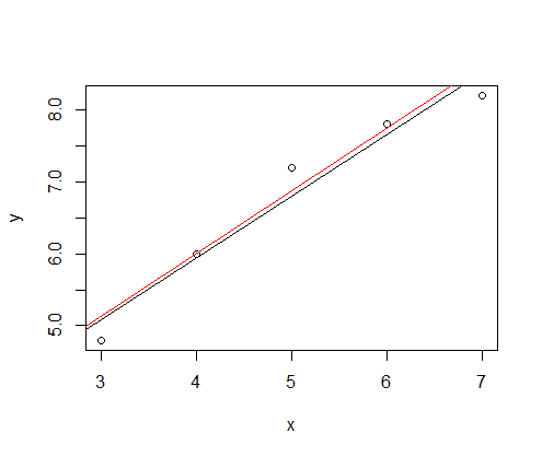
--빨간선이 비모수 방법
[edit]
23 오차 계산 #
이거 은근히 귀찮은데, 역시 만들어 놨군.
y <- c(4.17,5.58,5.18,6.11,4.50,4.61,5.17,4.53,5.33,5.14)
x <- c(4.81,4.17,4.41,3.59,5.87,3.83,6.03,4.89,4.32,4.69)
model <- lm(y ~ x)

library("DMwR")
regr.eval(y, fitted(model))
plot(x,y)
abline(model)
> regr.eval(y, fitted(model))
mae        mse       rmse       mape
0.41276110 0.24190200 0.49183534 0.08399855
[edit]
24 t-sql로 구현한 단순회귀분석 #
select
        (count(*)*sum(x*y)-(sum(x)*sum(y)))/(count(*)*sum(x*x)-(sum(x)*sum(x))) slope
    ,   avg(y)-((count(*)*sum(x*y))-(sum(x)*sum(y)))/((count(*)*sum(power(x,2)))-power(sum(x),2))*avg(x) intercept
from tbl_xy
create view v_test
as
select 98 x, 1 y union all
select 90, 2 union all
select 90, 3 union all
select 65, 4 union all
select 66, 5 union all
select 67, 6 union all
select 13, 7 union all
select 44, 8 union all
select 27, 9
go

declare
    @x nvarchar(255)
,   @y nvarchar(255)
,   @tablenm nvarchar(255)
,   @where nvarchar(1000)
,   @a nvarchar(255)
,   @b nvarchar(255)
,   @sql nvarchar(max);

set @x = 'x';
set @y = 'y';
set @tablenm = 'select * from v_test';
set @where = '';
set @sql = '
    declare
        @cnt int
    ,   @a decimal(38,5)
    ,   @b decimal(38,5)
    ,   @c decimal(38,5)
    ,   @d decimal(38,5)
    ,   @xavg decimal(38,5)
    ,   @yavg decimal(38,5)
    ,   @a1 decimal(38,5)
    ,   @b1 decimal(38,5);

    select
        @cnt = count(*)
    ,   @a = sum(convert(decimal(38,5), ' + @x + '))
    ,   @b = sum(convert(decimal(38,5), ' + @y + '))
    ,   @c = sum(convert(decimal(38,5), power(' + @x + ', 2)))
    ,   @d = sum(convert(decimal(38,5), ' + @x + '*' + @y + '))
    ,   @xavg = avg(convert(decimal(38,5), ' + @x + '))
    ,   @yavg = avg(convert(decimal(38,5), ' + @y + '))
    from (' + @tablenm + ') as t;

    set @a1 = ((@b*@c) - (@a*@d)) / (@cnt*@c - power(@a, 2));
    set @b1 = ((@cnt*@d) - (@a*@b)) / (@cnt*@c - power(@a, 2));

    select
        회귀식
    ,   round(r2, 4) [R-squared]
    ,   round(1-(1-r2)*(@cnt-1)/(@cnt-2),4) [Adjusted R-squared]
    ,   round(corr, 4) 상관계수
    from (
        select
            ''y = ''+ convert(nvarchar, @a1) + '' + '' + convert(nvarchar, @b1) +  ''x'' 회귀식
        ,   1 - var(' + @y + '-(@a1 + @b1*' + @x + ')) /
                    var(' + @y + ') r2
        ,   ((1.00/(@cnt - 1)*sum((' + @x + '-@xavg) * (' + @y + '-@yavg))) /
                    sqrt(var(' + @x + ') * var(' + @y + '))) corr
        from (' + @tablenm + ') as t
        where 1=1 ' + @where + '
    ) t

    select
        row_number() over(order by ' + @x + ') seq
    ,   ' + @x + ' x
    ,   ' + @y + ' y
    ,   power(' + @x + ', 2) x2
    ,   ' + @x + '*' + @y + ' xy
    ,   @a1 + @b1*' + @x + ' estimatedvalue_linear
    --,   @a1 * log(@a) + @b1 *' + @x + ' estimatedvalue_log
    ,   ' + @y + '-(@a1 + @b1*' + @x + ') diffvalue
    from (' + @tablenm + ') as t
    where 1=1 ' + @where + '
    order by 2;
    ';
print @sql;
exec(@sql);